Filling the Holes: How Match-Between-Runs Works, and How It Goes Wrong

By Max Burq, Dejan Stepec | September 7, 2026

If you have run the same samples through a mass spectrometer and opened the resulting table, you have seen the holes. A peptide is measured in seventeen of your twenty samples and simply absent from the other three. Nothing about the biology changed between those runs. The peptide was in the vial. The instrument just never got around to measuring it.

This post is about the technique used to fill those holes: match-between-runs. We will look at where it came from, why the literature has been uneasy about it for the past decade, and what we do to make it safer. No prior familiarity is assumed. A companion post covers what changes when the data are acquired by DIA.

What the Instrument Actually Measures

Start from the beginning.

The proteins in a sample are cut into peptides, which enter the instrument gradually over a period called the gradient. Depending on the experiment, that might be half an hour or a couple of hours. At any given moment, only some of the peptides are arriving. The instrument takes a survey scan, an MS1 scan, to measure the masses of the intact peptides present at that moment. Each detected peptide ion is a precursor.

That measurement tells you that something with a particular mass is there. It does not tell you what that something is. Different peptide sequences can have nearly the same mass, so mass alone is not enough to identify one.

To get the sequence, the instrument has to break the peptide apart. It isolates a precursor, fragments it, and records an MS2 scan containing the masses of the resulting fragments. Since peptides break at predictable points along their backbone, the pattern of fragments provides information about the amino acid sequence. Search software can then compare that spectrum with candidate sequences and score how well each one explains the observed fragments.

In other words, MS1 tells you something of this mass is here. MS2 gives you evidence for what that something is. A conventional identification is therefore a claim backed by a fragment spectrum.

Why DDA Leaves Holes

The problem starts with the way data-dependent acquisition (DDA) has to choose what to fragment.

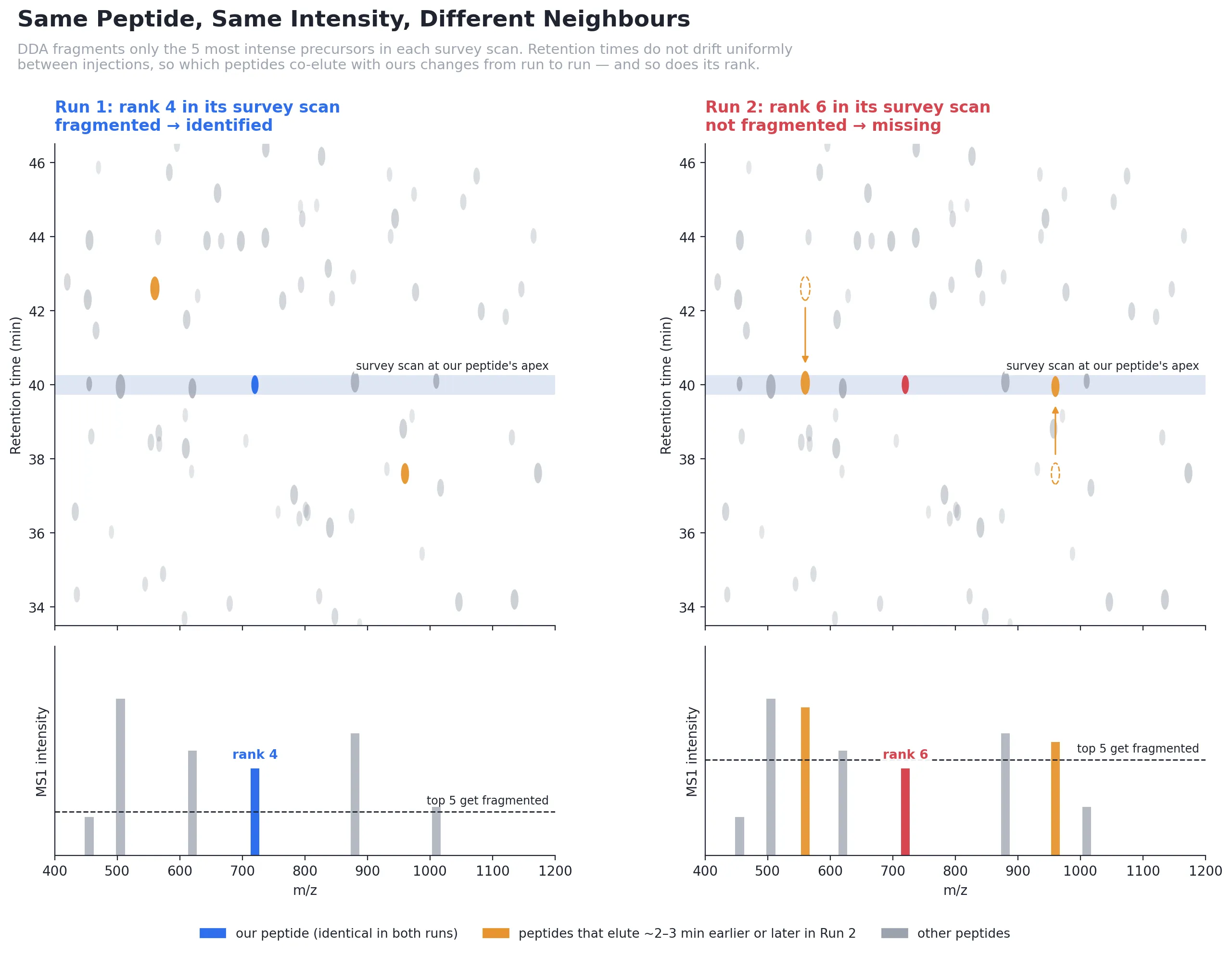
During a run, the instrument takes an MS1 survey and selects a handful of the most intense precursors — often the top ten or twenty. It fragments those one at a time, takes another survey, and repeats the process throughout the gradient.

There are far more peptides competing for attention than the instrument can fragment. Thousands can be co-eluting at a given moment, while only a few dozen can be selected before the chromatographic picture changes. And which peptides make the cut depends on what the instrument happens to see at that particular moment.

That makes selection both competitive and partly stochastic. A moderately abundant peptide might rank twelfth in one run and twenty-second in the next because of small differences in elution or ionization. In the first run, it gets fragmented and identified. In the second, it never gets selected.

Once that happens, the chain is straightforward: no selection means no fragmentation, no fragmentation means no MS2 spectrum, and no MS2 spectrum means no identification — regardless of how good the search software is.

That is where the holes come from. The peptide was present and may even have been detected at the MS1 level. It simply lost the scheduling lottery.

Match-Between-Runs: Borrowing an Identity

Match-between-runs is the obvious response. The technique, popularized by MaxQuant and now standard across the field, makes use of information that is already available elsewhere in the dataset. If a peptide was confidently identified in seventeen runs, there is good reason to think it is present in the other three as well.

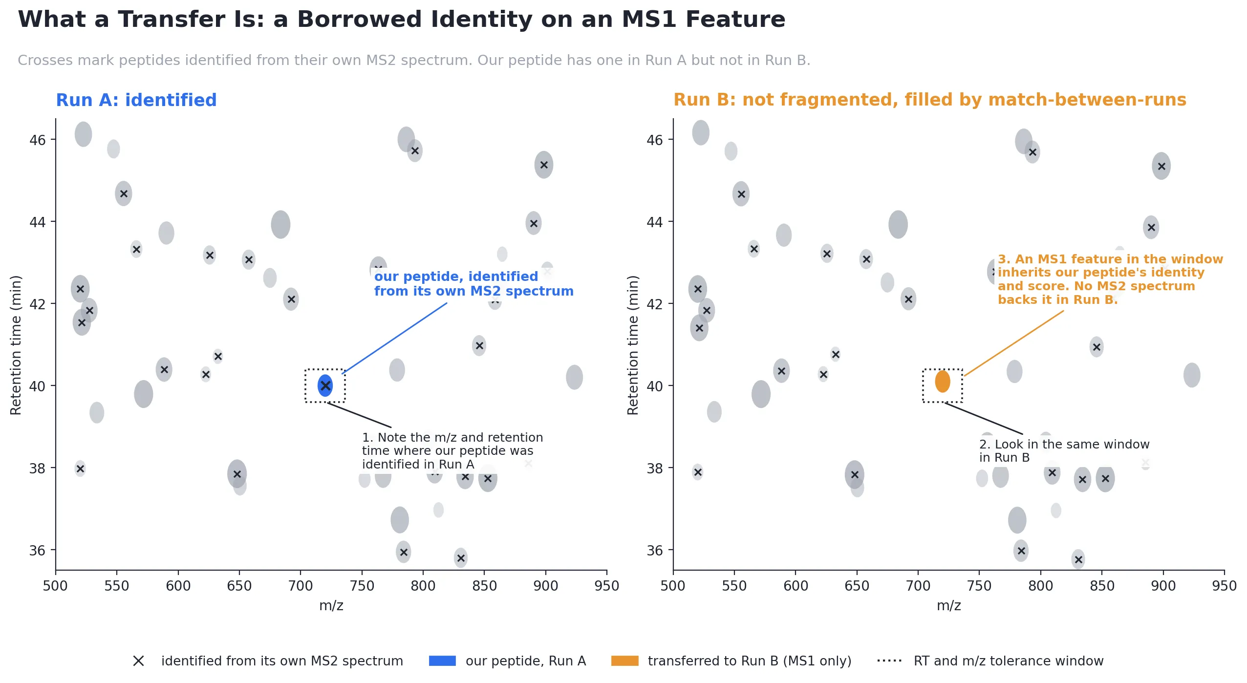
The first step is to put the runs onto the same retention-time scale. Retention times drift between injections, so the software fits a mapping between runs using peptides that were identified in both. Once that mapping exists, a peptide identified in run A but missing from run B has a predicted location in run B.

The software can then inspect the MS1 data around that location, looking for a peak with the expected mass and charge, and integrate it to obtain an intensity. The identity and confidence information from run A are attached to that signal, and the missing value is filled.

There is an important distinction hidden in that process. The measurement is an MS1 peak — a mass at a particular time — while the identity attached to it came from another run. The peptide sequence was never checked against fragment evidence in run B.

That is not simply a shortcut. It is a consequence of the acquisition method. The peptide is missing from run B precisely because the instrument did not fragment it there. There is no MS2 spectrum to recover after the fact. Given those constraints, matching on mass and retention time and transferring the existing identification is the best available option.

But the result is still different from an identification supported by an MS2 spectrum. With a conventional identification, you can pull up the fragment spectrum and inspect the evidence. For a transferred identification, the evidence in the target run is a mass, a retention time, and the assertion that this signal corresponds to an identification made somewhere else.

The Literature Has Been Uneasy About This

That distinction has practical consequences, and researchers have tested them.

One of the clearest tests uses a two-proteome experiment. You prepare some samples containing yeast and others containing no yeast at all, search them together, and turn match-between-runs on. If a yeast peptide appears in one of the yeast-free samples, you know that transfer is false: the way the samples were prepared gives you the ground truth.

Lim and colleagues did exactly this in 2019, using twenty yeast-containing and twenty yeast-free samples (J. Proteome Res. 18:4020–4026). Match-between-runs increased the total number of identifications by roughly 40%. At the same time, 44% of all identified yeast proteins were transferred into at least one sample that contained no yeast. That is a substantial number, and it goes a long way toward explaining why experienced users have been cautious about the feature.

There is another result from the same paper that matters just as much. Only about 2.7% of those false transfers made it into the final quantitative table, because downstream LFQ filtering in MaxQuant removed most of them.

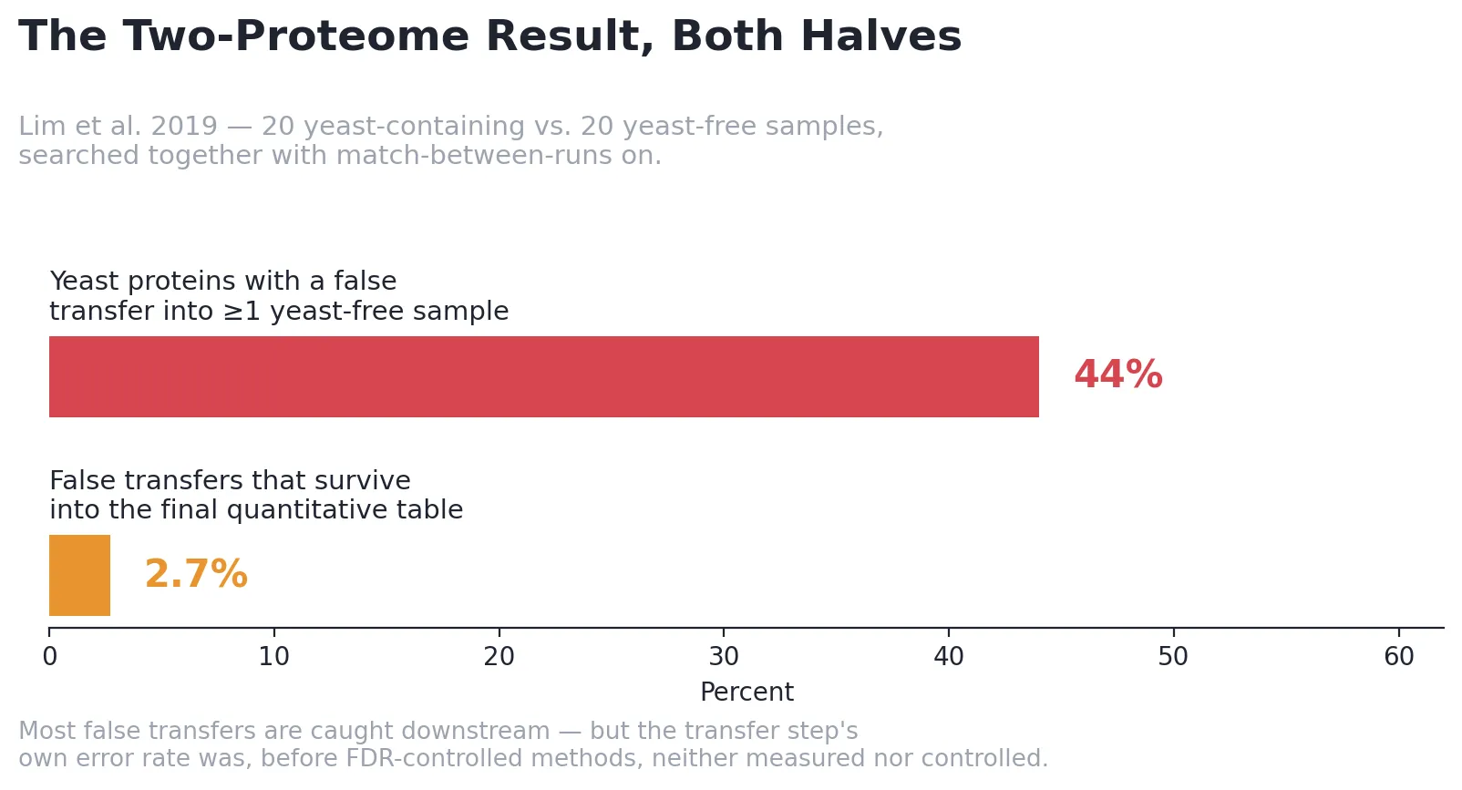
So the result is not simply that “match-between-runs is broken.” The more useful interpretation is that false transfers can be common at the transfer stage, most are removed later, and the transfer step itself does not tell you how many of the accepted matches are wrong.

That last part is the real difficulty. If you do not know the error rate of a step, you cannot properly account for it. You cannot tell a reviewer what that step costs you, and you cannot know whether its behaviour on your data is comparable to what someone else saw.

The response from the field has been to make transfers accountable. IonQuant introduced explicit FDR control for match-between-runs, modelling the distribution of transfer scores to estimate the fraction of accepted transfers that are incorrect (Yu, Haynes & Nesvizhskii, Mol. Cell. Proteomics 20:100077, 2021).

That is the direction we follow as well: a transfer should come with a measured error rate, rather than relying on a tolerance window and assuming it is good enough.

What We Do About It

Our DDA match-between-runs approach follows one basic principle: if the job needs a threshold, it should learn that threshold from its own data rather than inherit a fixed value tuned on somebody else’s instrument.

Only confident identifications may be sources. Before a peptide can be transferred, it must have been identified at 1% FDR in the source run. A transfer cannot be more reliable than the evidence it comes from.

A peptide must be identified in several runs before it may be transferred. This is the simplest safeguard, and it directly addresses the failure mode exposed by the two-proteome experiment. By default, we require a peptide to have been identified in at least three source runs.

A peptide seen only once is not allowed to propagate that single observation across the cohort. Instead, there needs to be corroboration from several independent runs before the identification can be transferred.

There is one practical complication: the requirement is capped at one less than the total number of runs in the job. The run receiving a transfer cannot also serve as a source for that same transfer. Without the cap, a three-run experiment would require a peptide to already be present in all three runs, leaving nothing for match-between-runs to fill. Small cohorts therefore get a weaker but still functional version of the feature rather than one that silently does nothing. A two-run job is the weakest case, because there can only be one source and therefore no cross-run corroboration.

Retention-time alignment is fitted robustly. The mapping between two runs is based on confidently shared identifications. After the initial fit, outliers are removed and the alignment is fitted again. This prevents a small number of genuinely shifted peptides from distorting the mapping for everything else. If an alignment cannot be fitted reliably, the run can simply be skipped instead of using a bad map to make transfers.

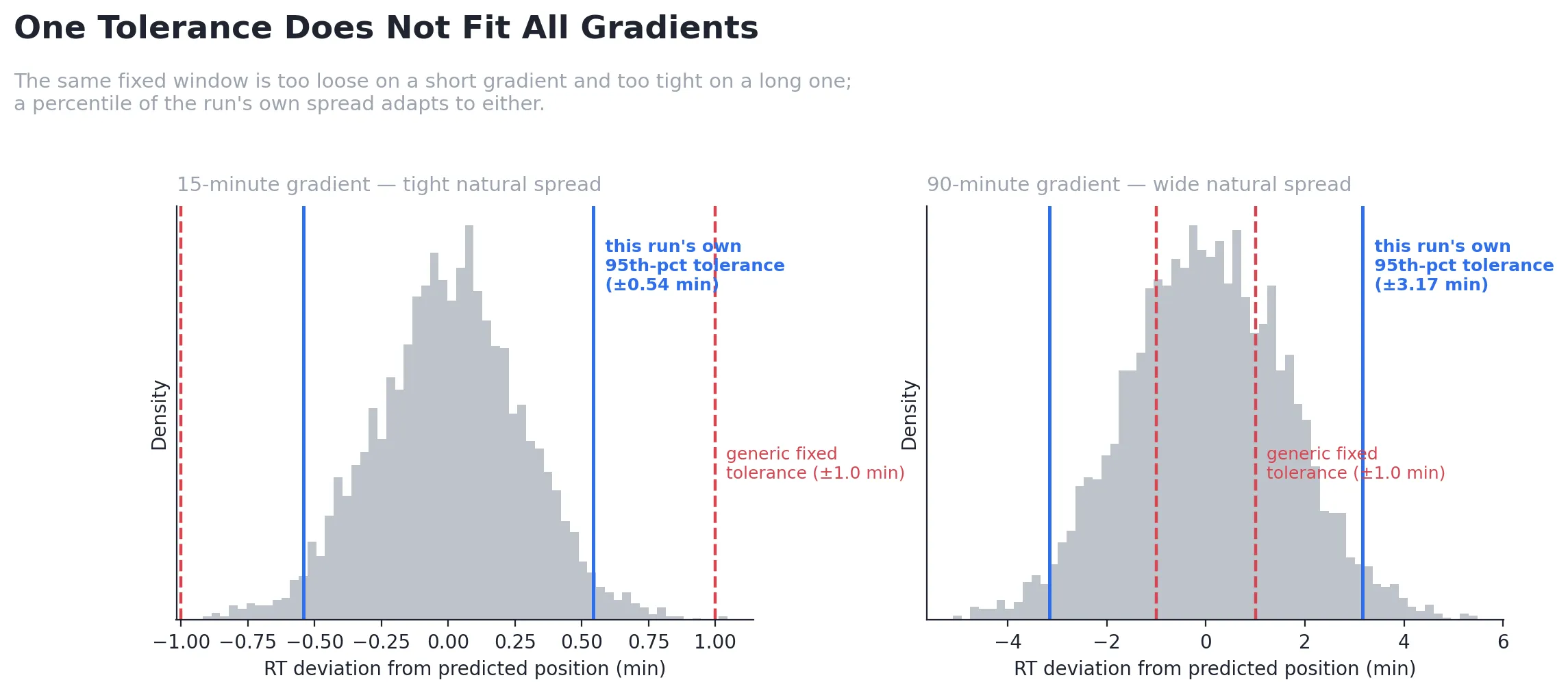
The retention-time gate is calibrated per run, from that run’s own data. A fixed tolerance in minutes is a poor fit for experiments with different gradient lengths. A tolerance that is reasonable on a 15-minute gradient does not necessarily mean the same thing on a 90-minute gradient.

Instead, each run provides its own reference. The method looks at how far the run’s identified features are from the scans that triggered them, and uses a percentile of that observed spread to set the transfer tolerance. A candidate that falls farther from its predicted location than the run’s normal variation is therefore treated as anomalous relative to that run, rather than relative to a fixed number chosen in advance.

The acceptance model is trained on labelled transfers generated by the job itself. This is the part we think matters most. The model is a logistic regression over features of the MS1 peak the transfer lands on: its shape (width, fit to an elution profile, prominence over background), its isotope evidence (M1/M0 ratio, co-elution of the isotope traces, signal one isotope below that points to another species), its mass error, its distance from the predicted retention time, its intensity, and how clearly it dominates the other peaks in the window.

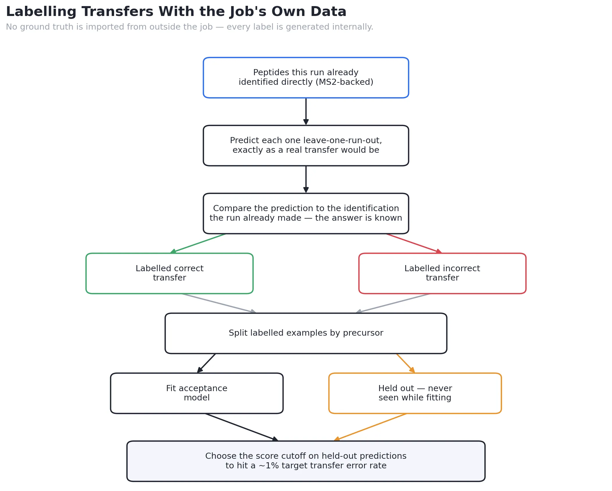
The candidate set includes peptides that the target run actually identified. We then predict those identifications in a leave-one-run-out fashion, the same way we would predict a genuine transfer. Because the peptide’s own retention time is left out when making the prediction, it cannot simply validate itself.

At the same time, we already know the correct answer for these cases: the target run did identify the peptide. That turns them into labelled examples that the job can use to learn what a successful transfer looks like, without having to import ground truth from another experiment.

This gives us something a simple tolerance-based approach cannot provide: the job can estimate its own wrong-transfer rate and use that estimate to set the acceptance cutoff. We fit the acceptance model on the labelled transfers and choose the score cutoff to target an error rate of about 1%.

The cutoff itself is chosen out-of-fold, using predictions from data the model was not fitted on. The split is done by precursor rather than by row. That matters because an in-sample cutoff can look excellent during validation while failing to achieve the intended error rate on real transfers. We have measured that failure ourselves.

Decoy candidates travel alongside real ones, which gives the transfer step a way to estimate its error rate using the same general principle used for estimating identification error elsewhere in the pipeline.

When a job is too small to calibrate, it says so by degrading. If there are not enough labelled examples to train the model reliably, it falls back to permissive behaviour rather than rejecting everything. A small job therefore gets less protection; it does not silently produce an empty result.

The Honest Limitation

These safeguards make DDA transfers considerably more accountable than a fixed tolerance window. They do not, however, change what a transferred identification actually is.

In DDA, a transferred identification is supported by an MS1 measurement — a mass at a retention time — rather than fragment evidence in the run where it is reported. We can measure how often that goes wrong and control it, and that is what we do. But we cannot show you the spectrum, because there isn’t one.

That limitation belongs to the acquisition method rather than the algorithm. Change the way the data are acquired, and the situation changes. That is the subject of the companion post on DIA, where every recovered peptide retains a spectrum that can be audited.

---

References:

• Lim, M. Y. et al. 2019. Evaluating false transfer rates from the match-between-runs algorithm with a two-proteome model. J. Proteome Res. 18:4020–4026.
• Yu, F., Haynes, S. E. & Nesvizhskii, A. I. 2021. IonQuant enables accurate and sensitive label-free quantification with FDR-controlled match-between-runs. Mol. Cell. Proteomics 20:100077.
• Cox, J. et al. 2014. Accurate proteome-wide label-free quantification by delayed normalization and maximal peptide ratio extraction (MaxLFQ). Mol. Cell. Proteomics 13:2513–2526.